Introducing the Riverlane Roadmap: Three basic steps to decoder success 

We have posted our first arXiv pre-print that dives deep into our current generation decoder (DD1) for quantum error correction.

Here I explain what our decoder is, what functionality it unlocks for qubit manufacturers and users, as well as our vision for what next steps are needed to reach fault-tolerance.

A quick refresher on Quantum Error Correction (QEC) codes and decoders

A QEC code uses many noisy qubits to build a more reliable logical qubit. Provided the qubits, code and decoder meet some noise threshold requirements, the more qubits we use the more reliable (higher fidelity) our logical qubit is.

Performing QEC produces a continuous data stream from repeated rounds of measurements, which are designed to detect the presence of qubit errors. This information must then be processed by a sophisticated algorithmic process that we call decoding.

QEC has gone from theory to practice, with several landmark demonstrations in the last couple of years. Using superconducting qubits, ETH Zurich demonstrated a good quality 17 qubit QEC code. Later, a Google experiment showed that a 49 qubit QEC code does indeed improve on the reliability of the ETH 17 qubit QEC code. Additional, exciting QEC results have been shown with other qubit modalities, including ion traps and neutral atoms.

Both the ETH Zurich and Google experiments relied on decoding off-line meaning the measurement results were collected and decoding happened later (possibly days or weeks later), rather than in real-time with data collection. This is OK for these early QEC demonstrations as they show we can build the qubit components of logical quantum memory.

But for a useful quantum computer, we don’t only require reliable logical quantum memories but also need the capability to perform logical operations between logical qubits. And this means we need real-time decoding because we need to decode each logic gate to ensure it works reliably before proceeding to the next logic gate.

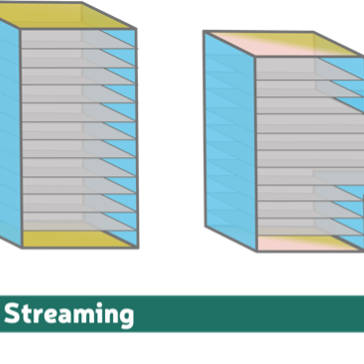
Figure 1: The real-time decoding problem as a sequence of important milestones. See Figures 2, 5 and 6 for details.

Decoding in real-time is a huge challenge for fast quantum computers (like superconducting) as a million rounds of measurement results are produced every second in superconducting qubits. If we don’t decode fast enough, we encounter an exponentially growing backlog of syndrome data. And for useful quantum computing, we need to push the scale of the decoder up to so-called Teraquop decoding speeds.

For a true real-time decoder, we want it to do three things (very quickly):

1. Deterministic: the decoder needs to respond promptly at well determined times (which sounds simple but many computer architectures like CPUs are liable to respond at their leisure);
2. Streaming: the decoder must process continuous streams of measurement results as they arrive, not after an experiment is finished;
3. Adaptive: the decoder must respond to earlier decoding decisions through tight integration with the control systems, which are a fundamental component of the quantum error correction stack.

These three features will guide our discussion of current and future generations of Riverlane decoders, as well as the corresponding experiments they unlock.

What we’ve already built and what it unlocks now (DD1)

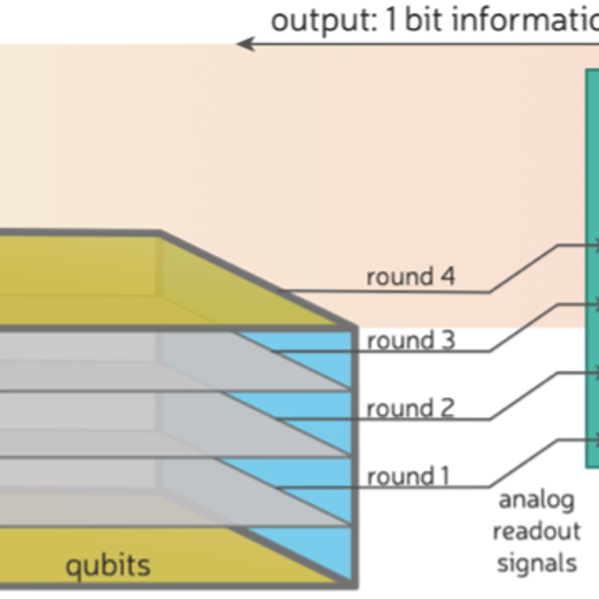
Figure 2: Schematic of a quantum error correction experiment supported by DD1. Time runs from the bottom upwards. From left to right: a control system sends a series of pulses to qubits; subsequent rounds of QEC are illustrated by 2D planes; each QEC round generates a collection of analog pulses; a readout system converts analog pulses to digital syndrome information; a decoder instance starts processing all of the syndrome data as a single batch. To time the speed of the decoder, we start a clock once the last round of QEC has been performed until the decoder gives its final output bit.

Our current decoder (DD1) enables quantum memory demonstrations that unlock the first real-time feature, deterministic decoding (1), for a QEC code called the surface code (this is what the Google and Zurich teams used).

It needs to be fast, which is why we developed the Collision Clustering algorithm, which works by growing clusters of errors and quickly evaluating whether they collide or not (see the pre-print for all the details!).

Lots of our partners are interested in QEC codes other than the surface code or using decoders more focused on improving logical fidelity than achieving real-time decoding. And for these partners we have, in parallel, developed software decoding tools to (off-line) solve a wider range of QEC tasks, but that is a story for another day.

To implement Collision Clustering, we coded it up in a very low-level language called Verilog. This enables us to load (or flash) the Verilog code onto a computer called an FPGA – a Field Programmable Gate Array. FPGAs are big, chunky integrated circuits (see Figure 3) that can be reprogrammed (“Programmed” in the “Field”) to solve a specialised task. They have many advantages including that they behave deterministically (1) ensuring that they always complete tasks in a timely manner.

While there are lots of excellent software packages available for decoding, they are coded in higher-level languages suitable for CPUs and are not necessarily going to behave deterministically.

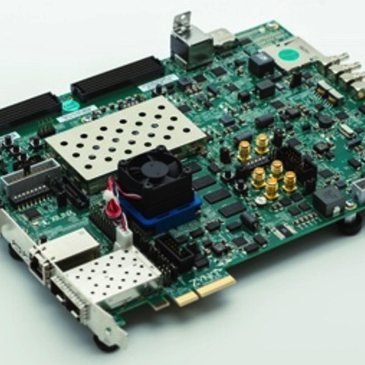
Figure 3: An example Field Programmable Gate Array (FPGA) shown on a common hardware implementation used in quantum computing stacks, especially as part of the control systems. DD1 can be flashed onto an FPGA using a small percentage of resources, often alongside existing control components.

FPGAs are a useful platform as every quantum computer in the world currently uses them to generate pulses to control qubits. So, our decoder easily slots in alongside existing infrastructures. Indeed, you could use our decoder for up to 1,000 qubits and it would still use less than 6% of the resources on an FPGA (based on a Xilinx). So, it could even share space with an FPGA without needing any new hardware purchases.  Our arXiv preprint includes benchmarking results of our decoder based on such an FPGA implementation.

In the longer term, the cost and bulk of FPGAs means that large quantum computers will need to shift to using Application Specific Integration Circuits (ASICs) for their decoders and control systems. An ASIC looks a lot like the CPU inside your laptop or phone, but it is tailored for a specific task and behaves more deterministically like an FPGA.

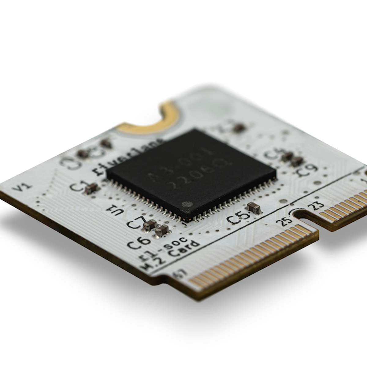
Figure 4: An ASIC (15mm²) taped out by Riverlane implementing an earlier prototype (DD0A).

Compared to an FPGA, an ASIC is faster, much cheaper (pennies per unit rather than tens of thousands of pounds) and much lower in power consumption. The catch is that building an ASIC requires a foundry to “tape-out” your design onto a silicon chip. Every new generation or update to your decoder needs a new tape-out.  So, they aren’t as quickly deployable since most current quantum computers use FPGAs for their control systems.

In summary, FPGAs are convenient now, but ASICs are the future. This is why our current decoder is also tape-out ready, and we’ve completed a test tape-out of an earlier generation: DD0A, which is the world’s first decoder ASIC.  DD0A is a demonstration chip with DD1A due to be produced in 2024.

Even without the tape-out process complete, our Verilog code enables us to benchmark the expected ASIC performance and our preprint gives all the details of these results.

By producing the world’s first decoder ASIC and with the release of our decode IP, we are providing the short-term and long-term decode solutions for quantum hardware companies.

Our vision for what next?

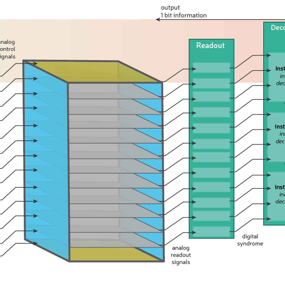
Figure 5: A space-time illustration of a quantum error correction experiment following the conventions of Figure 1. The main difference here is that decoder instances start processing batches of syndrome data (called windows – more on this below) while the experiment is still running. Each instance/window must wait for the previous logical operation to finish before it can start its task. The relevant response time is from the end of the experiment until the final decoder output is produced. We know we have avoided the backlog problem if we can execute an unlimited number of QEC rounds, while never exceeding a constant, maximum response time.

Our current generation decoder has the right foundations for real-time decoding, and we are currently building more sophisticated functionality to fully support large-scale error corrected quantum computing.

Firstly, the current decoder takes the output of a whole QEC experiment (including preparing the logical qubit and finally reading it out) and decodes it as a single batch of all of the syndrome data generated by that experiment. It completes this task quickly and in a reliable amount of time (it behaves deterministically). But it isn’t continuously decoding a stream of data!

A streaming decoder must break up the syndrome data into batches, called windows. We can start decoding a window once we’ve performed all the relevant measurements. Then, once this window has been decoded, we can move onto the next window of data and start decoding it.

However, decoding is a complex holistic problem and can’t neatly be parcelled up into a completely independent window. So, we need each of the windows to overlap and we also need to build extra functionality in our decoder to reconcile what happens when these windows overlap.

If your decoder is fast enough, we can keep pace with the syndrome data by only using one decoder instance at a time, a so-called sliding window (aka overlapping window) approach.

And after that?

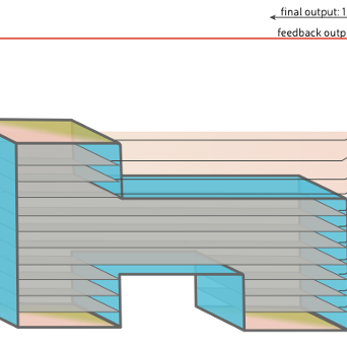
Figure 6: A space-time illustration of a quantum error correction experiment following the conventions of Figure 1 and Figure 4. This experiment starts (at the bottom) with two separate logical qubits, then a logical operation is performed by merging the patches, then we shrink down to a standard patch size, and then measure in an adaptive basis. Since the decoding problem is broken up into three stages, we only have to wait until the second stage has finished its workload before triggers the feedback message to the control system (shown by a red arrow).

Once we can continuously decode a logical quantum memory, the next step forward is to demonstrate decoding of a logical quantum computer. The fundamental differences here are that:

1. The decoder must support decoding while performing logical operations;
2. The decoder needs to be adaptive (with the real-time decoding feature 3) so that it can feedback decisions about what to do before the next logical operation.

In Figure 6, we show the simplest two-logical qubit computation primitive where real-time decoding becomes truly essential. The figure shows a simple teleportation and logical readout experiment. This is the simplest primitive where it is crucial to adapt the third logical operation (measurement) depending on the decoding results of the second logical operation (patch merging).